
Gozynta Mobius 3.1 Feature Release

 by Andrew Hamlin
My first experience with Kanban was in 2012 or 2013 when, as manager of a 10-person sustaining engineering team, I needed to organize software delivery against internal SLAs. We were responsible for resolving Support issues escalated to Engineering. The time frames and priorities changed daily, if not hourly. Managing via Scrum with sprints was simply not adaptive enough. I found a great primer from Jesper Boeg on Kanban and over a month or so reinvented our development and release process around Kanban metrics. The turn around was dramatic and the team wonderfully successful.
I will leave further evangelising to others. If you are interested, the Agile Alliance has published a case study of Siemens Health Services that is a great representation of applying these techniques.
This article shows how to build the sets of metrics and charts to perform probabilistic forecasting. Forecasting can be used to answer either of the following questions.
There are many products available to use Kanban and Lean metrics for your software development. However, I put this together because switching tools can be a major undertaking and not always an option. So, if you want to make use of forecasting based on Monte Carlo simulations but do not want to invest in time and money to completely switch your project management tools, here I will explain the steps I used to generate these results using Google Sheets are my spreadsheet.
The basic Kanban/Lean metrics are:
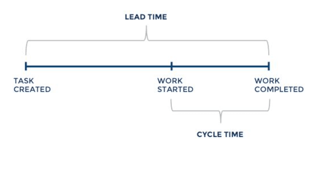
Cycle time is the duration of time it takes to work on and complete an item.
Throughput is the count of items completed during a time period.
Work in progress is the count of items being worked on during a time period.
The diagram used to view these three metrics is the cumulative flow diagram. Because this article is focused on building a forecast using a spreadsheet, I have omitted the CFD from here. If you are not familiar, you can find many resources online. Kanbanize has a one such article.
The calculation of flow through a system is simply an application of Little's Law. You can determine any of the three metrics, as follow:
WIP = Throughput * Cycle time
Or,
Throughput = WIP / Cycletime
Or,
Cycletime = WIP / Throughput
Lead time is the entire amount of time it takes an item to move through the system, not just the amount of time spent actively working on the item. For example, with 10 items in a queue your team won't begin working on the 10th item right away. The 10th item will sit ready to be worked on for a period of time. The lead time accounts for the time spent waiting, in addition to the actual cycle time.
The fundamental idea of optimizing flow through your system is limiting your work in progress. This is the easiest way to decrease the cycle time and increase the throughput. A great visual demonstration of this is on YouTube created by Michel Grootjans, Explaining team flow.
However, lead time and improving your flow are beyond the scope of this article. Let's get straight to how you can use these metrics to forecast your delivery.
I am using Google Sheets as my spreadsheet and the calculations make heavy use of the QUERY function. The QUERY function uses Google's Visualization API Query language.
For the forecasting you will need to capture the start and end dates of work on each item.
The steps in this article will cover using work days rather than calendar days, that is days excluding weekends (and holidays). You can choose what is right for your teams, I prefer normalizing to work days (maybe just out of habit). Either will work, as long as you and your stakeholders are aware of the base unit of time.
The cycle time in work days calculation uses the NETWORKDAYS function:
=NETWORKDAYS('start date', 'closed date', [holidays])
Resulting two columns:
| A | B | |-------------+------------| | closed date | cycle time | | 2021-08-02 | 2 | | 2021-08-03 | 3 | | 2021-08-04 | 3 | | 2021-08-04 | 1 |
Everything else in the forecasting can be built from these values.
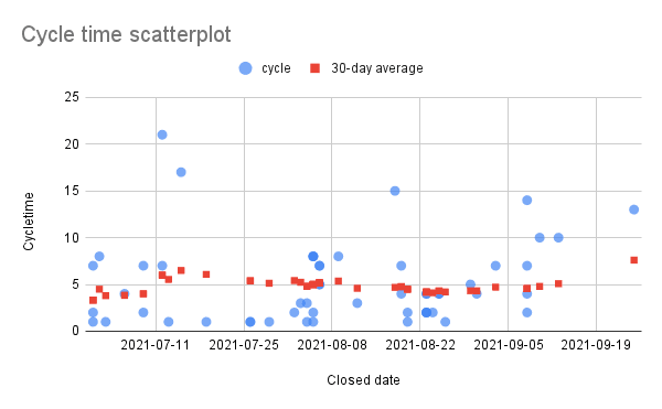
A scatterplot shows the distribution of your cycle times. It is also useful to view the trend of cycletimes by calculating the rolling average.
Calculate the rolling average on 30 days with a SELECT statement finding all cycletimes (column B) that were closed between closed date and 30 days earlier. This uses the Visualization API date expression.
=AVERAGE(QUERY(A$2:B,
         "SELECT B WHERE A > date '"&TEXT(A2-30, "yyyy-mm-dd")
         &"' AND A <= date '"&TEXT(A2, "yyyy-mm-dd")&"'", -1))
Note that the QUERY range locks the range to begin at row 2, $2 and sets the optional headers argument to -1, meaning the selected range has no header rows. Alternatively, you can lock row 1, $1 and provide headers argument 1 so the query language will recognize row 1 as headers of the range.
| A | B | C |
|---|---|---|
| closed date | cycle time | rolling average |
| 2021-08-02 | 2 | 5.416666667 |
| 2021-08-03 | 3 | 5.230769231 |
| 2021-08-04 | 3 | 4.8 |
| 2021-08-04 | 1 | 4.8 |
Now you can create a scatterplot chart including a secondary rolling average plot. In this example data you can clearly see that the 30-day rolling average started to tick back up (e.g. slow down) in September. This is a trend you can then discuss with the team to better understand.
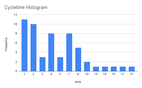
Create a pivot table to view a histogram of cycletimes. Set the pivot table row as 'cycle time' and the values as 'COUNTA(cycle time)'.
| cycle time | COUNTA(cycle time) |
|---|---|
| 1 | 11 |
| 2 | 10 |
| 3 | 3 |
| 4 | 8 |
Then, create a bar chart.
Determine the likelihood of future items' cycle times by using the PERCENTILE formula to calculate a range of possible cycletimes. The formula refers to the sheet comtaining the cycle time data 'cycle time'!$B2:$B and the cell above the formula B1:
=PERCENTILE('cycle time'!$B$2:$B,B1)
Note that the range is locked on column B that is the cycle time column. Allowing you to drag the formula horizontally while referring to the percentages in the preceding row.
| A | B | C | D | E | F |
|---|---|---|---|---|---|
| Probability | 0.25 | 0.5 | 0.75 | 0.85 | 0.98 |
| Cycletime | 2 | 4 | 7 | 8 | 16.84 |
Now you can see that 85% of the time the cycle time for a single item is less than or equal to 8 days.
Next, to forecast either of your outcomes, When or How Many, you need to calculate your throughput.
Again, Throughput is simply the number of items completed during a time period, and I like to calculate based on work days rather than calendar days.
The simplest formula for thoughput relies on knowing the count of items completed between your start and end dates.
We will go back to the NETWORKDAYS formula to determine the workdays in our time period.
=NETWORKDAYS('start date', 'closed date', [holidays])
The item completed count can simply be the COUNTA of the cycletime columns or ROWS in the range. If your data table includes more than your target range, you can use the QUERY or FILTER functions.
=COUNTA('cycle time'!B$2:B)
And the throughput is simple the result of count of items divided by the workdays in the period.
=B5/B4
| A | B |
|---|---|
| Period Start | 2021-07-01 |
| Period End | 2021-09-25 |
| Workdays in Period | 62 |
| Completed in Period | 55 |
| Throughput (count/workday) | 0.8870967742 |
This calculation however has one drawback in that you can' calculate the standard deviation of your throughput, and the STDEV is required for running a Monte Carlo simulation.
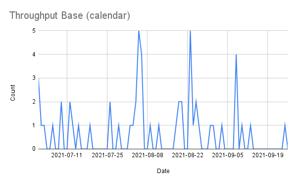
I am interested in calculating workday throughput but first I want to visualize the base throughput.
Create a data table including all the dates of your time period. Enter your start date in format yyyy-mm-dd, then drag the cell down until your end date. Then, use the QUERY formula to extract a count of items closed per date.
=IFERROR(ROWS(QUERY('cycle time'!A$2:B,
         "SELECT B WHERE A = date '"&TEXT(A2, "yyyy-mm-dd")&"'", -1)), 0)
Here I exclude the header row using A$2:B in the range and -1 as optional headers argument.
| A | B |
|---|---|
| Date | Count |
| 2021-08-01 | 0 |
| 2021-08-02 | 1 |
| 2021-08-03 | 1 |
| 2021-08-04 | 2 |
| 2021-08-05 | 5 |
Now, creating a line chart will show the throughput over our time period, including the weekends. This nice from a human view point to remember that we should take advantage of our weekends and holidays!
In order to make prediction based on workdays, we need to transform this calendar view to workdays. Here is a cool little formula that will generate the workday dates, and then we can use a slightly more complex QUERY formula to count all the items closed on a given workday.
The formula in two columns looks like this. Simple drag the cells down to include your target range.
| Date | Count per workday |
| 2021-07-01 | =IFERROR(ROWS(QUERY('cycle time'!A$2:B$56, "SELECT B WHERE A >= date '"&TEXT(D2, "yyyy-mm-dd")&"' AND A < date '"&TEXT(WORKDAY(D2, 1),"yyyy-mm-dd")&"'", -1)), 0) |
| =WORKDAY(D$2,ROW(D1)) | =IFERROR(ROWS(QUERY('cycle time'!A$2:B$56, "SELECT B WHERE A >= date '"&TEXT(D3, "yyyy-mm-dd")&"' AND A < date '"&TEXT(WORKDAY(D3, 1),"yyyy-mm-dd")&"'", -1)), 0) |
The Date column formula uses the relative positioning of the ROW to calculate the number of workdays WORKDAY(D$2, ROW(D1)) from the start date 2021-07-01.
The Count per workday formula selects all rows where the closed date Column A is greater than or equal to the date and less than the next workday WORKDAY(D2, 1). And is wrapped in an IFERROR that returns zero if no items were closed within that date range. Any items completed outside of a workday will be counted in the preceding workday. For example, an item closed on Saturday will increment Friday's count by one.
The result is a data table excluding weekends (and holidays, if you fill in the optional holidays range).
| D | E | |------------+-------------------| | Date | Count per workday | | 2021-08-05 | 5 | | 2021-08-06 | 4 | | 2021-08-09 | 1 | | 2021-08-10 | 0 |
This workday data now comtains enough detail to accurately calculate the throughput average (mean) and also standard deviation.
| workdays mean | =AVERAGE('throughput base'!E2:E) |
| workdays stdev | =STDEV('throughput base'!E2:E) |
| workdays median | =MEDIAN('throughput base'!E2:E) |
| workdays mode | =MODE('throughput base'!E2:E) |
Resulting data table give you all the values needs to perform a Monte Carlo simulation based on throughput.
| workdays mean | 0.8870967742 | | workdays stdev | 1.229485281 | | workdays median | 0.5 | | workdays mode | 0 |
You can also generate a probability table of your throughput, similar to the cycle time probability. Again, using the PERCENTILE formula as described earlier.
| Probability | 0.25 | 0.5 | 0.75 | 0.85 | 0.98 |
|---|---|---|---|---|---|
| Throughput | 0 | 0.5 | 1 | 2 | 4.78 |
If you are wondering why the Mode and the 98% are included, you can read about thin-tailed versus fat-tailed distributions. In short, thin-tailed distributions yield higher accuracy predictions.
Now that you have all your data tables setup, it is time to run the simulations.
First, you want to know when you will complete 30 items, based on historical throughput.
Simulation: When will we complete N items? Throughput (mean): 0.8870967742 Throughput (stdev): 1.229485281 Start date: 2021-10-11 Item count: 30
The Monte Carlo simulation is simply the division of your count of items by the NORMINV formula, repeated 10s of thousands of times.
| A | B |
|---|---|
| Throughput | Workdays |
=NORMINV(RAND(), mean, stdev) | =ROUNDUP(count/A1) |
What I have done in the spreadsheet is create a seperate sheet, and drag this formula down 1000 rows. Then copy and paste columns A:B, paste values only, 10 times across, yielding 10K results. Then on another sheet combine the results into 1 large static table.
In Google Sheets, the combination of ranges is down by using the ={range;range;range;...} expression.
={'data'!D1:E1000;'data'!F1:G1000;'data'!H1:I1000;'data'!J1:K1000;'data'!L1:M1000;'data'!N1:O1000;'data'!P1:Q1000;'data'!R1:S1000;'data'!T1:U1000;'data'!V1:W1000}
The throughput simulation distribution can be viewed by creating a pivot table on the resulting workday count colum. This explains the use of the ROUNDUP function.
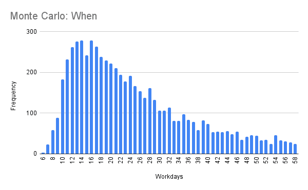
Use the when data table $B14:$B and the facts table above, and the PERCENTILE formula to calculate your probability forecast.
| Probability | 0.25 |
| Workdays | =PERCENTILE($B14:$B,B6) |
| End date | =WORKDAY($B3,B$7) |
Resulting in
| Probability | 0.25 | 0.5 | 0.75 | 0.85 | 0.98 |
|---|---|---|---|---|---|
| Workdays | 8 | 19 | 37 | 57 | 418.02 |
| End date | 10/21/2021 | 11/5/2021 | 12/1/2021 | 12/29/2021 | 5/18/2023 |
Second, you want to know how many items you will complete by a certain end date.
Simulation: How many items can we complete by date D? Throughput (mean): 0.8870967742 Start date: 2021-10-11 End date: 2021-11-19 Workdays in period: 30
Again, use the NETWORKDAYS function calculate the days in the time period.
This simulation is simply the multiplication of the workdays in your time period and the NORMINV formula, repeated 10K times.
| A | B | | Throughput | Item count | | =NORMINV(RAND(), main, stdev) | =ROUNDUP(workdays * A1) |
What I have done in the spreadsheet is create a seperate sheet, and drag this formula down 1000 rows. Then copy and paste columns A:B, paste values only, 10 times across, yielding 10K results. Then on another sheet combine the results into 1 large static table.
In Google Sheets, the combination of ranges is down by using the ={range;range;range;...} expression.
={'data'!D1:E1000;'data'!F1:G1000;'data'!H1:I1000;'data'!J1:K1000;'data'!L1:M1000;'data'!N1:O1000;'data'!P1:Q1000;'data'!R1:S1000;'data'!T1:U1000;'data'!V1:W1000}
The throughput simulation distribution can be viewed by creating a pivot table on the resulting item count colum. This explains the use of the ROUNDUP function.
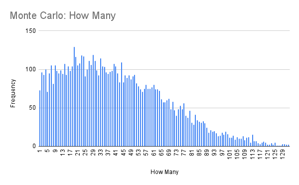
Use the when data table $B14:$B and the facts table above, and the PERCENTILE formula to calculate your probability forecast.
| Probability | 0.25 |
| Items | =PERCENTILE(QUERY($B15:$B, "SELECT B WHERE B > 0", -1), 1-B$6) |
Note: The percentage is inverted, 1-$B$6, because it is more likely we will complete less items rather than more items. It doesn't make sense to say we have a 25% chance to complete 20 items, but a 75% to complete 60.
Resulting in
| Probability | 0.25 | 0.5 | 0.75 | 0.85 | 0.98 |
|---|---|---|---|---|---|
| Items | 60 | 38 | 20 | 13 | 2 |
And that's it. I hope this is helpful to you.

